Analysis with R and BigQuery
Computing on the BigQuery side; making correlation matrices
In this example, we are going to compute a correlation matrix (or co-expression) entirely on the BigQuery side. Since we’re in R-land, we can easily visualize the matrix as a heatmap. We are also going to query for gene lists using Gene Ontology annotation, and access the End Points API to get a list of samples.
Loading libraries
require(bigrquery, quietly = TRUE) || install.packages('bigrquery',verbose = FALSE)
require(httpuv, quietly = TRUE) || install.packages('httpuv',verbose=FALSE)
require(ggplot2, quietly = TRUE) || install.packages('ggplot2',verbose = FALSE)
The ISB-CGC R Examples Package
The collection of examples can be found at: https://github.com/isb-cgc/examples-R
To install the package, we use the devtools package.
require(devtools, quietly = TRUE) || install.packages('devtools',verbose = FALSE)
require(ISBCGCExamples, quietly = TRUE) || install_github("isb-cgc/examples-R", build_vignettes=F)
If you needed to install any of the packages, remember, you still need to import it!
Your project ID
You will be using your own project ID. At certain points in the code, it will be necessary to complete the code.
my_cloud_project   = "your_project_id"
tcga_data_set      = "TCGA_hg38_data_v0"
First query
Now let’s see if things are working.
bigrquery::list_tables("isb-cgc", tcga_data_set)
Using BigQuery to compute correlation matrices
A correlation matrix using gene expression is going to take the correlation between each pair of genes. Usually, this matrix can then be clustered to discover gene modules.
In this query, we’re going to use the BigQuery CORR function (one of the many built-in mathematical functions) to compute a Pearson’s correlation.
You can find all the function information at: https://cloud.google.com/bigquery/query-reference
The general structure of the query is going to be:
select
  genes and correlation
from
  subtable with genes and samples of interest
joined to
  same subtable of genes and samples
q <- "
    SELECT
      a.gene_name AS gene1,
      b.gene_name AS gene2,
      CORR(a.HTSeq__FPKM,
        b.HTSeq__FPKM) AS corr
    FROM (
      SELECT
        *
      FROM
        `isb-cgc.TCGA_hg38_data_v0.RNAseq_Gene_Expression`
      WHERE
        gene_name IN ('APLN',
          'CCL26',
          'IL19',
          'IL37')
        AND project_short_name = 'TCGA-COAD' ) AS a
    JOIN (
      SELECT
        *
      FROM
        `isb-cgc.TCGA_hg38_data_v0.RNAseq_Gene_Expression`
      WHERE
        gene_name IN ('APLN',
          'CCL26',
          'IL19',
          'IL37')
        AND project_short_name = 'TCGA-COAD' ) AS b
    ON
      a.aliquot_barcode = b.aliquot_barcode
    GROUP BY
      gene1,
      gene2"

corrs <- query_exec(q,my_cloud_project, use_legacy_sql=F)

# transform to a matrix, and give it rownames
library(tidyr)
corrmat <- spread(corrs, gene1, corr)
rownames(corrmat) <- corrmat$gene2

# visualize the matrix
library(pheatmap)
pheatmap(corrmat[,-1])
It’s easy to make a couple changes to this query, enabling a correlation matrix per study. Try it!
Getting a list of high variance genes
When we make queries from R, the results come back as a data.frame. Let’s use the GO annotation, and get a list of genes that are related to the immune system. The GO Annotation table is found in the genome_reference data set, and GO:0006955 references the immune response.
q <- "
SELECT
  DB_Object_Symbol
FROM
  `isb-cgc.genome_reference.GO_Annotations`
WHERE
  GO_ID = 'GO:0006955'"

query_exec(q, my_cloud_project, use_legacy_sql=F)
That query returns 472 genes. But let’s suppose we want the top 50 by coefficient of variance.
q <- "
    SELECT
      gene_name,
      STDDEV(HTSeq__FPKM+1) / AVG(HTSeq__FPKM+1) AS cv
    FROM
      `isb-cgc.TCGA_hg38_data_v0.RNAseq_Gene_Expression`
    WHERE
      gene_name IN (
      SELECT
        DB_Object_Symbol
      FROM
        `isb-cgc.genome_reference.GO_Annotations`
      WHERE
        GO_ID = 'GO:0006955')
      AND project_short_name = 'TCGA-BRCA'
    GROUP BY
      gene_name
    ORDER BY
      cv DESC
    LIMIT
      50"

result <- query_exec(q, my_cloud_project, use_legacy_sql=F)
genes <- result$gene_name
Now we have a list of genes that we can carry to further analysis.
Getting a list of samples from the endpoints
From R we can access the cohorts we created using the web app. To do that we use the End Points API. The API is essentially a set of html requests. A small wrapper is included as part of the isb-cgc examples-R package.
https://github.com/isb-cgc/examples-R/blob/master/inst/doc/Working_With_Barcode_Lists.md
To get started, import the ISBCGCExamples library.
library(ISBCGCExamples)
The first step is creating a token. This token contains your authentication status, and lets the service know about what information is available to you.
my_token <- isb_init()
To get a listing of the previously created cohorts, we can use the list_cohorts function that takes a token, and returns a list with items including ‘count’, ‘items’, ‘kind’, and ‘etag’. The count shows the number of saved cohorts and the items contains information about the cohorts.
# first get a list of my saved cohorts.
my_cohorts <- list_cohorts(my_token)
names(my_cohorts)

# to get the names of my saved cohorts
lapply(my_cohorts$items, function(x) x$name)
Now that we have the cohort IDs, we can collect the various barcodes contained in the cohort. These include patient barcodes, sample barcodes, and aliquot barcodes. To do this, we can use the barcodes_from_cohort function.
HERE I’m using my cohort #4, but change this to whatever you have saved.
# get the cohort IDs
my_cohort_id <- lapply(my_cohorts$items, function(x) x$id)[[4]]

# then ping the endpoints with the cohort ID
my_barcodes <- cohort_barcodes(my_cohort_id, my_token)
names(my_barcodes)
The object returned from barcodes_from_cohort is again a list, this time with elements ‘cohort_id’, ‘sample_count’, ‘case_count’, ‘cases’, and ‘samples’. The cases and samples elements are also lists, but lists of cases or sample barcodes.
samples <- unlist(my_barcodes$samples)
# 836 samples
Programmatically constructing Queries
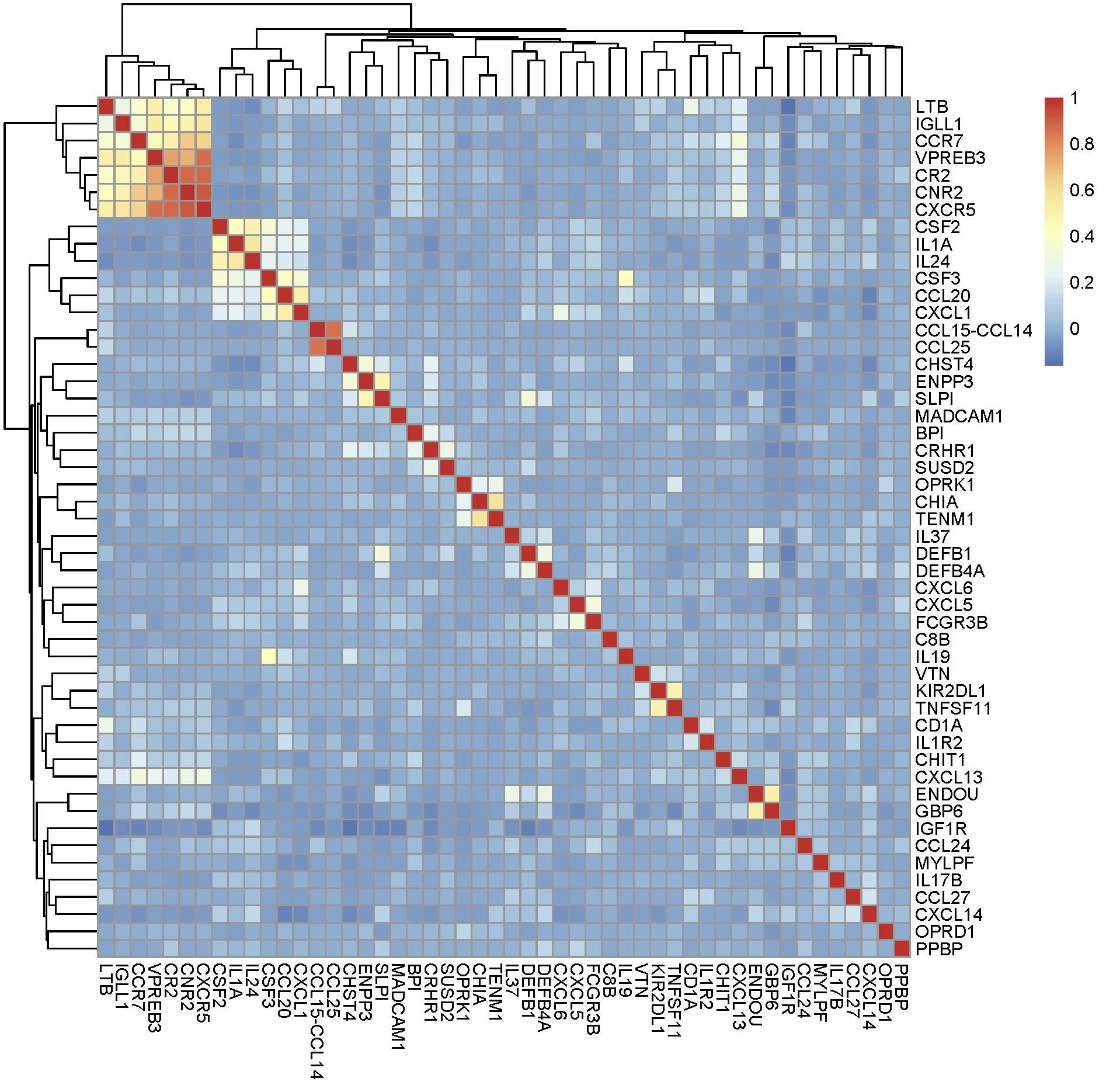
One of the great things about working in a scripting environment, is that our analysis – the queries – we write, can be constructed programmatically. That makes it easy to apply the same structured queries to many questions. But also we can incorporate long lists of samples or genes into a query.
#function for formatting lists..
sqf <- function(x) {
    paste("('",paste(x, collapse="','"),"')", sep="")
}

q <- paste("
SELECT
  a.gene_name as gene1,
  b.gene_name as gene2,
  CORR(a.HTSeq__FPKM, b.HTSeq__FPKM) as corr
FROM (
  SELECT
    *
  FROM
    `isb-cgc.TCGA_hg38_data_v0.RNAseq_Gene_Expression`
  WHERE
    gene_name IN ", sqf(genes), "
    AND sample_barcode IN ", sqf(samples), "
  ) AS a
JOIN (
  SELECT
    *
  FROM
    `isb-cgc.TCGA_hg38_data_v0.RNAseq_Gene_Expression`
  WHERE
    gene_name IN ", sqf(genes), "
    AND sample_barcode IN ", sqf(samples), "
  ) AS b
ON
  a.aliquot_barcode = b.aliquot_barcode
GROUP BY
  gene1,
  gene2", sep=" ")

corrs <- query_exec(q,my_cloud_project, use_legacy_sql=F)

# transform to a matrix, and give it rownames
library(tidyr)
corrmat <- spread(corrs, gene1, corr)
rownames(corrmat) <- corrmat$gene2

# visualize the matrix
library(pheatmap)
pheatmap(corrmat[,-1])
From Lists to Matrices
Transform gexp_affected_genes_df into a gexp-by-samples feature matrix
gexp_fm = tidyr::spread(gexp_affected_genes,HGNC_gene_symbol,normalized_count)

gexp_fm[1:5,1:5]