Analysis Using BigQuery, R & Bioconductor
In this tutorial, we are interested in analyzing gene expression and protein abundance differences between two types of TCGA kidney cancers, Kidney Renal Clear Cell Carcinoma (KIRC) and Kidney Renal Papillary Carcinoma (KIRP). We will build a cohort of patients with these cancer types and extract their respective gene expression and protein abundance data using Google BigQuery.
Note
An interactive step-by-step version of this tutorial can also be found on our homepage here.
This tutorial demonstrates how to:
Identify tables of interest using the ISB-CGC BigQuery Table Search UI
Navigate to tables in the Google BigQuery Console directly from the ISB-CGC BigQuery Table Search
Build and run queries in the Google BigQuery Console
Link to R notebooks in the Google AI Platform for data interrogation and plot visualization
Use Bioconductor packages designed for TCGA data on ISB-CGC BigQuery tables
There are no prerequisites for using the ISB-CGC BigQuery Table Search, but in order to use the ISB-CGC tables in the Google Cloud BigQuery Console and within an R program, you’ll need to have a Google Cloud Platform project and have linked it to the ISB-CGC BigQuery tables. Please see these sections of the ISB-CGC documentation for guidance:
Click on the screenshots below to enlarge them.
Using the ISB-CGC BigQuery Table Search
Navigate to the ISB-CGC homepage: https://isb-cgc.org and click on the Launch icon in the BigQuery Table Search box.

Let’s search for ISB-CGC hosted BigQuery tables that contain information for TCGA gene expression, protein expression and clinical data. We want to build a cohort of TCGA patients for which both gene expression and protein abundance data exists. Enter TCGA in the Program filter and Clinical Data, Gene Expression, and Protein Expression in the Data Type filter. To see the table schema of the clinical table, click on the (+) icon.
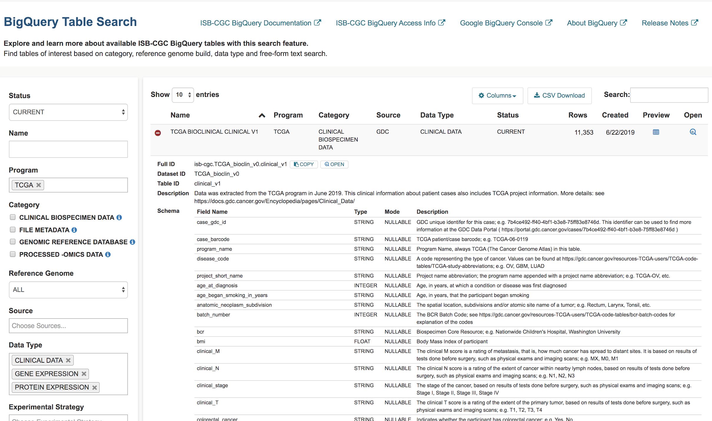
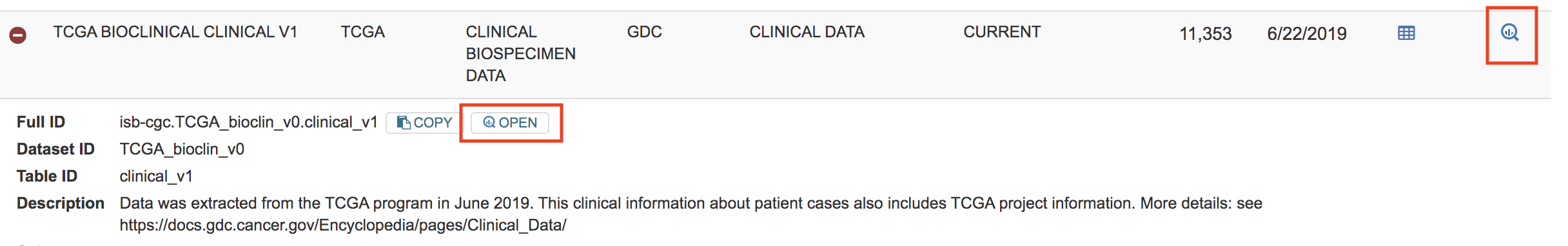
Navigate to the Google Cloud Platform (GCP) BigQuery Console by clicking on the “open” button under the table preview or on the “magnifying glass” icon on the right hand side of the Table Search row.
Using the Google Cloud BigQuery Console
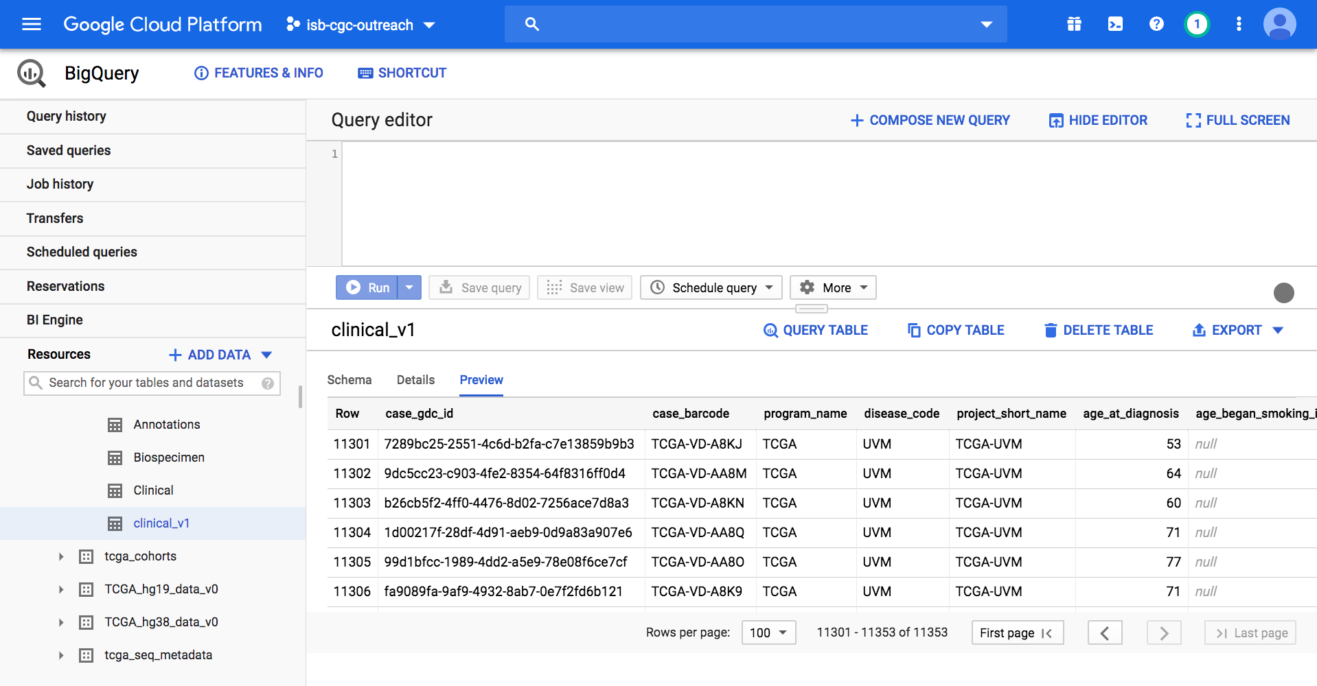
On the GCP BigQuery Console we can preview the table, look at the schema, and perform queries. The image below shows the preview of the contents of the TCGA Clinical BigQuery table.
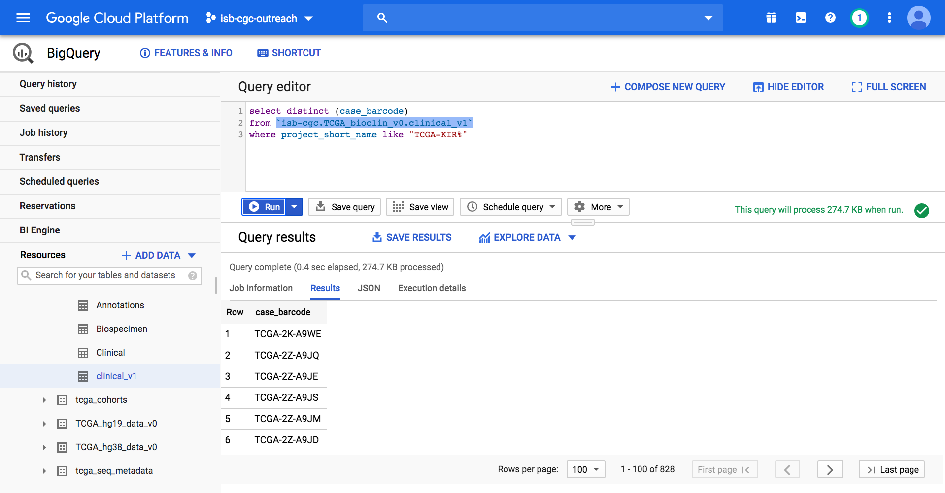
Here’s a short SQL query (that completes in 0.3 seconds) which identifies how many patients there are with TCGA kidney cancers. Enter this SQL query in the BigQuery Console and click Run:
SELECT distinct (case_barcode)
FROM `isb-cgc.TCGA_bioclin_v0.clinical_v1`
WHERE project_short_name LIKE "TCGA-KIR%"
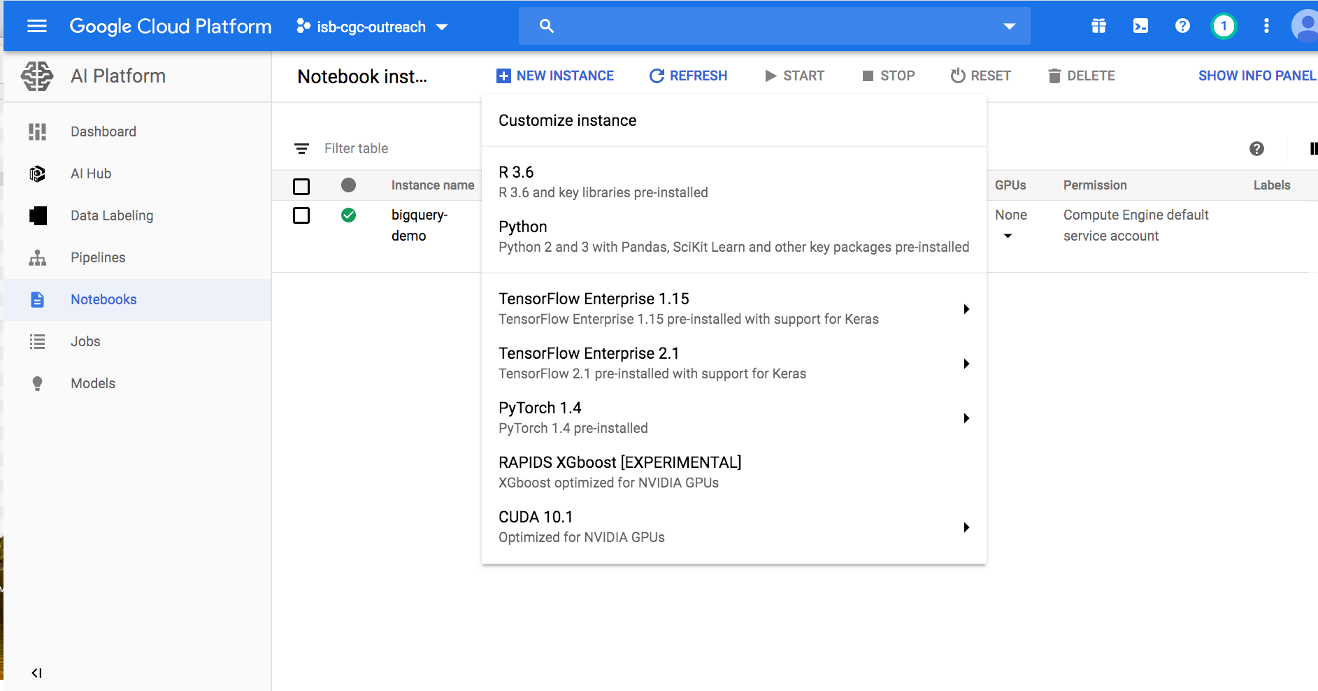
Using a Google Cloud AI Platform R Notebook and Bioconductor
From here, we can use either R or Python to perform higher level analyses. In this example, we will be running an R notebook in the Google Cloud AI Platform Notebooks environment. If you prefer, you can run this example in a local R environment instead.
To use Google Cloud AI Platform Notebooks, from the Google Cloud Platform Navigation menu (on the left), select AI Platform -> Notebooks under the Artificial Intelligence section.

Notebooks can be created in both R or Python. We’ll create our notebook in R.
The Google Cloud AI platform R notebook environment looks very similar to other Jupyter notebook environments. Users can create interactive R notebooks or simpler R console notebooks.
Enter or copy each block into the R terminal. Click Run after each block to see the results.
install.packages("bigrquery")
library(bigrquery)
project <- "your project" #Replace with your project name
# Query the clinical table for our cohort.
# Retrieve Age at Diagnosis and Clinical Stage for Kidney Cancer data.
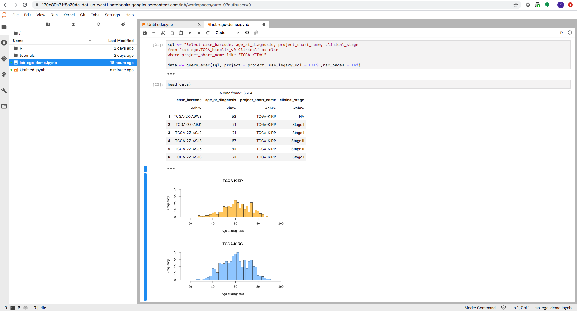
sql <- "Select case_barcode, age_at_diagnosis, project_short_name, clinical_stage
from `isb-cgc.TCGA_bioclin_v0.Clinical` as clin
where project_short_name like 'TCGA-KIR%'"
clinical_tbl <- bq_project_query (project, query = sql) #Put data in temporary BQ table
clinical_data <- bq_table_download(clinical_tbl) #Put data into a dataframe
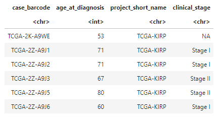
head(clinical_data)
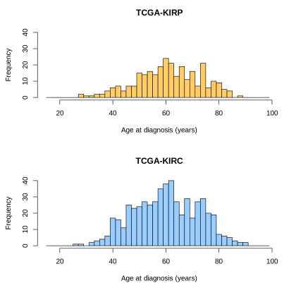
# Plot two histograms of age of diagnosis data of our cohort.
layout(matrix(1:2, 2, 1))
hist(clinical_data[clinical_data$project_short_name == "TCGA-KIRP",]$age_at_diagnosis,
    xlim=c(15,100), ylim=c(0,40), breaks=seq(15,100,2),
    col="#FFCC66", main='TCGA-KIRP', xlab='Age at diagnosis (years)')

hist(clinical_data[clinical_data$project_short_name == "TCGA-KIRC",]$age_at_diagnosis,
    xlim=c(15,100), ylim=c(0,40), breaks=seq(15,100,2),
    col="#99CCFF", main='TCGA-KIRC', xlab='Age at diagnosis (years)')
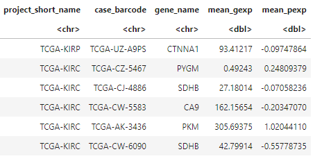
# Create SQL query to retrieve the mean gene expression and mean protein expression per project/case.
# Load it into a dataframe.
sql_expression <- "with gexp as (
    select project_short_name, case_barcode, gene_name, avg(HTSeq__FPKM) as mean_gexp
    from `isb-cgc.TCGA_hg38_data_v0.RNAseq_Gene_Expression`
    where project_short_name like 'TCGA-KIR%' and gene_type = 'protein_coding'
    group by project_short_name, case_barcode, gene_name
), pexp as (
    select project_short_name, case_barcode, gene_name, avg(protein_expression) as mean_pexp
    from `isb-cgc.TCGA_hg38_data_v0.Protein_Expression`
    where project_short_name like 'TCGA-KIR%'
    group by project_short_name, case_barcode, gene_name
)
select gexp.project_short_name, gexp.case_barcode, gexp.gene_name, gexp.mean_gexp, pexp.mean_pexp
from gexp inner join pexp
on gexp.project_short_name = pexp.project_short_name
  and gexp.case_barcode = pexp.case_barcode
  and gexp.gene_name = pexp.gene_name"

expression_data <- bq_table_download(bq_project_query (project, query = sql_expression)) #Put data into a dataframe
head(expression_data)
# Determine the number of cases from each project.
length(unique(expression_data$case_barcode[expression_data$project_short_name == "TCGA-KIRP"]))
length(unique(expression_data$case_barcode[expression_data$project_short_name == "TCGA-KIRC"]))

#Create a dataframe that lists all the cases.
expression_data$id <- paste(expression_data$project_short_name, expression_data$case_barcode, sep='.')
cases <- unique(expression_data$id)
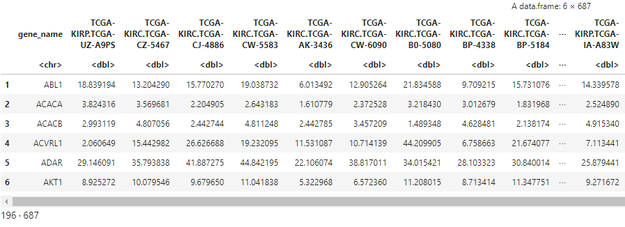
# Transform the expression_data data frame, so that columns are samples, rows are genes.
list_exp <- lapply(cases, function(case){
temp <- expression_data[expression_data$id == case, c('gene_name', 'mean_gexp')]
names(temp) <- c('gene_name', case)
return(temp)
})
gene_exps <- Reduce(function(x, y) merge(x, y, all=T, by="gene_name"), list_exp)
head(gene_exps)
dim(gene_exps)
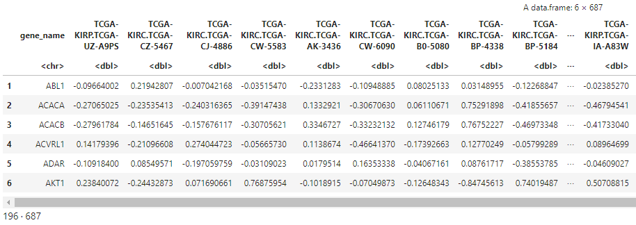
# Perform the same transform for protein abundance.
  list_abun <- lapply(cases, function(case){
      temp <- expression_data[expression_data$id == case, c('gene_name', 'mean_pexp')]
      names(temp) <- c('gene_name', case)
      return(temp)
  })
  pep_abun <- Reduce(function(x, y) merge(x, y, all=T, by="gene_name"), list_abun)
  head(pep_abun)
  dim(pep_abun)
# Separate the cohorts (types of kidney cancer) into two dataframes and
# generate a scatterplot of gene expression and protein abundance.
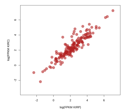
# Gene expression first.
exp_p <- gene_exps[,grep('KIRP', names(gene_exps))]
exp_c <- gene_exps[,grep('KIRC', names(gene_exps))]
plot(log(rowMeans(exp_p)), log(rowMeans(exp_c)),
xlab='log(FPKM KIRP)', ylab='log(FPKM KIRC)',
xlim=c(-3.5,7.5), ylim=c(-3.5,7.5), pch=19, cex=2,
col=rgb(178,34,34,max=255,alpha=150))
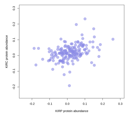
# Peptide expression second.
abun_p <- pep_abun[,grep('KIRP', names(pep_abun))]
abun_c <- pep_abun[,grep('KIRC', names(pep_abun))]
plot(rowMeans(abun_p), rowMeans(abun_c),
   xlab='KIRP protein abundance', ylab="KIRC protein abundance",
   xlim=c(-0.25,0.3), ylim=c(-0.25,0.3), pch=19, cex=2,
   col=rgb(140,140,230,max=255,alpha=150))
# Load the Bioconductor package maftools, which has capabilities to summarize,
# analyze and visualize Mutation Annotation Format (MAF) data.
install.packages("maftools")
library("maftools")
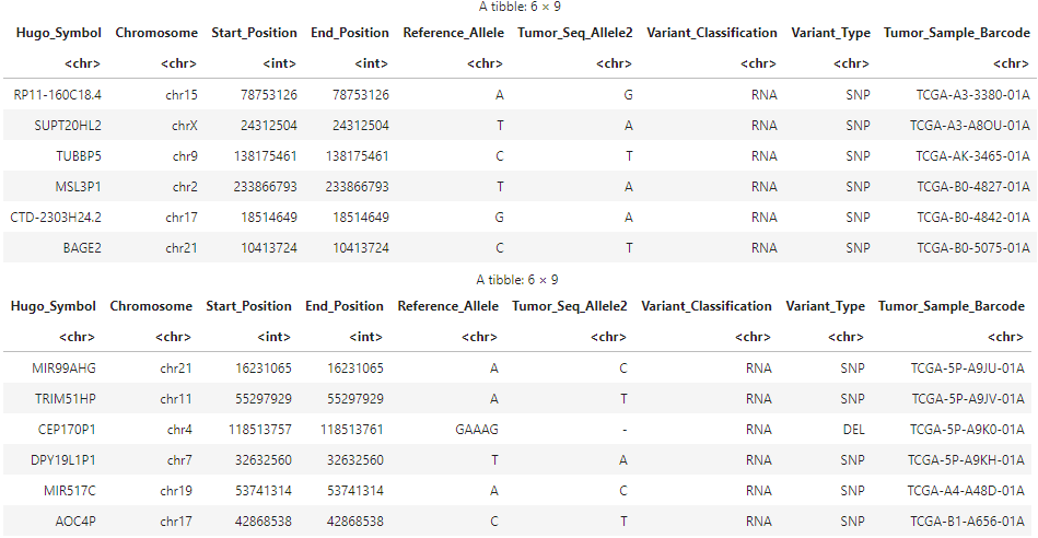
# Use BigQuery to load TCGA somatic mutation data for our cancers of interest.
sql_kirc<-"SELECT Hugo_Symbol, Chromosome, Start_Position, End_Position, Reference_Allele,
Tumor_Seq_Allele2, Variant_Classification, Variant_Type, sample_barcode_tumor FROM
`isb-cgc.TCGA_hg38_data_v0.Somatic_Mutation` WHERE project_short_name = 'TCGA-KIRC'"

sql_kirp<-"SELECT Hugo_Symbol, Chromosome, Start_Position, End_Position, Reference_Allele,
Tumor_Seq_Allele2, Variant_Classification, Variant_Type, sample_barcode_tumor FROM
`isb-cgc.TCGA_hg38_data_v0.Somatic_Mutation` WHERE project_short_name = 'TCGA-KIRP'"

maf_kirc <- bq_table_download(bq_project_query (project, query = sql_kirc)) #Put data into a dataframe
maf_kirp <- bq_table_download(bq_project_query (project, query = sql_kirp)) #Put data into a dataframe

#Rename column 9 to the field name required by maftools.
colnames(maf_kirc)[9] <- "Tumor_Sample_Barcode"
colnames(maf_kirp)[9] <- "Tumor_Sample_Barcode"

head(maf_kirc)
head(maf_kirp)
# Convert data frames to maftools objects.
kirc <- read.maf(maf_kirc)
kirp <- read.maf(maf_kirp)
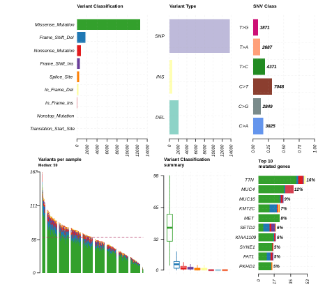
# Leverage maftools plotting functionality.
plotmafSummary(maf = kirp, rmOutlier = TRUE, addStat = 'median', dashboard = TRUE, titvRaw = FALSE)
plotmafSummary(maf = kirc, rmOutlier = TRUE, addStat = 'median', dashboard = TRUE, titvRaw = FALSE)
Here is the MAF Plot Summary for Kidney Renal Papillary Carcinoma.
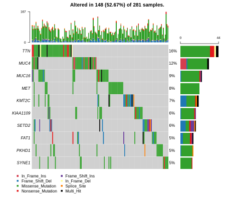
oncoplot(maf = kirp, top = 10)
oncoplot(maf = kirc, top = 10)
Here is the oncoplot for Kidney Renal Papillary Carcinoma.